Algorithm Analysis
Algorithms are the most important and durable part of computer science because they can be studied in a language- and machine-independent way. This means we need techniques that let us compare the efficiency of algorithms without implementing them. Our two most important tools are
- the RAM model of computation and
- the asymptotic analysis of computational complexity (i.e., big-)
The RAM model of computation
Machine-independent algorithm design depends upon a hypothetical computer called the Random Access Machine, or RAM. Under this model of computation, we are confronted with a computer where:
- One time step
- Simple operations (assumption 1): Each simple operation (
+,*,-,=,if, call) takes exactly one time step. - Memory access (assumption 3): Each memory access takes exactly one time step. Furthermore, we have as much memory as we need. The RAM model takes no notice of whether an item is in cache or on the disk.
- Simple operations (assumption 1): Each simple operation (
- Several time steps
- Non-simple operations (assumption 2): Loops and subroutines are not considered simple operations. Instead, they are the composition of many single-step operations. It makes no sense for sort to be a single-step operation, since sorting 1,000,000 items will certainly take much longer than sorting ten items. The time it takes to run through a loop or execute a subprogram depends upon the number of loop iterations or the specific nature of the subprogram.
Under the RAM model, we measure run time by counting the number of steps an algorithm takes on a given problem instance. If we assume that our RAM executes a given number of steps per second, this operation count converts naturally to the actual running time.
The RAM is a simple model of how computers perform. Perhaps it sounds too simple. After all, multiplying two numbers takes more time than adding two numbers on most processors, which violates the first assumption of the model. Fancy compiler loop unrolling and hyperthreading may well violate the second assumption. And certainly memory-access times differ greatly depending on where your data sits in the storage hierarchy. This makes us zero for three on the truth of our basic assumptions.
And yet, despite these objections, the RAM proves an excellent model for understanding how an algorithm will perform on a real computer. It strikes a fine balance by capturing the essential behavior of computers while being simple to work with. We use the RAM model because it is useful in practice.
Every model in science has a size range over which it is useful. Take, for example, the model that the Earth is flat. You might argue that this is a bad model, since it is quite well established that the Earth is round. But, when laying the foundation of a house, the flat Earth model is sufficiently accurate that it can be reliably used. It is so much easier to manipulate a flat-Earth model that it is inconceivable that you would try to think spherically when you don't have to.
The same situation is true with the RAM model of computation. We make an abstraction that is generally very useful. It is difficult to design an algorithm where the RAM model gives you substantially misleading results. The robustness of this model enables us to analyze algorithms in a machine-independent way.
Best-case, worse-case, and average-case complexity
Using the RAM model of computation, we can count how many steps our algorithm takes on any given input instance by executing it. However, to understand how good or bad an algorithm is in general, we must know how it works over all possible instances.
To understand the notions of the best, worst, and average-case complexity, think about running an algorithm over all possible instances of data that can be fed to it. For the problem of sorting, the set of possible input instances includes every possible arrangement of keys, for all possible values of . We can represent each input instance as a point on a graph where the -axis represents the size of the input problem (for sorting, the number of items to sort), and the -axis denotes the number of steps taken by the algorithm in this instance:
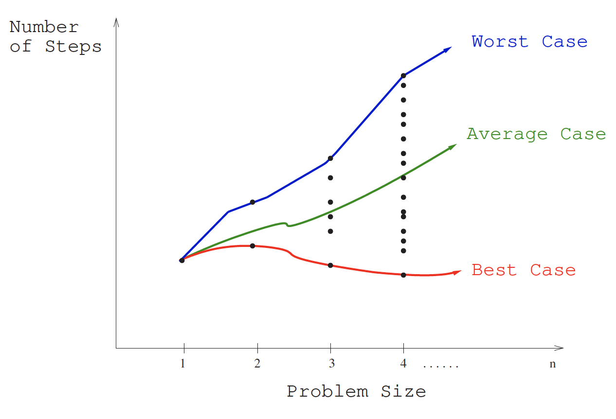
These points naturally align themselves into columns, because only integers represent possible input sizes (e.g., it makes no sense to sort 10.57 items). We can define three interesting functions over the plot of these points:
- Worst-case: The worst-case complexity of the algorithm is the function defined by the maximum number of steps taken in any instance of size . This represents the curve passing through the highest point in each column.
- Best-case: The best-case complexity of the algorithm is the function defined by the minimum number of steps taken in any instance of size . This represents the curve passing through the lowest point of each column.
- Average-case: The average-case complexity or expected time of the algorithm, which is the function defined by the average number of steps over all instances of size .
The worst-case complexity generally proves to be most useful of these three measures in practice. Many people find this counterintuitive. To illustrate why, try to project what will happen if you bring $n into a casino to gamble. The best case, that you walk out owning the place, is so unlikely that you should not even think about it. The worst case, that you lose all $n, is easy to calculate and distressingly likely to happen.
The average case, that the typical bettor loses 87.32% of the money that he or she brings to the casino, is both difficult to establish and its meaning subject to debate. What exactly does average mean? Stupid people lose more than smart people, so are you smarter or stupider than the average person, and by how much? Card counters at blackjack do better on average than customers who accept three or more free drinks. We avoid all these complexities and obtain a very useful result by considering the worst case.
That said, average-case analysis for expected running time will prove very important with respect to randomized algorithms, which use random numbers to make decisions within the algorithm.
The Big Oh notation
The best-case, worst-case, and average-case time complexities for any given algorithm are numerical functions over the size of possible problem instances. However, it is very difficult to work precisely with these functions, because they tend to:
Have too many bumps — An algorithm such as binary search typically runs a bit faster for arrays of size exactly (where is an integer), because the array partitions work out nicely. This detail is not particularly important, but it warns us that the exact time complexity function for any algorithm is liable to be very complicated, with lots of little up and down bumps as shown below:
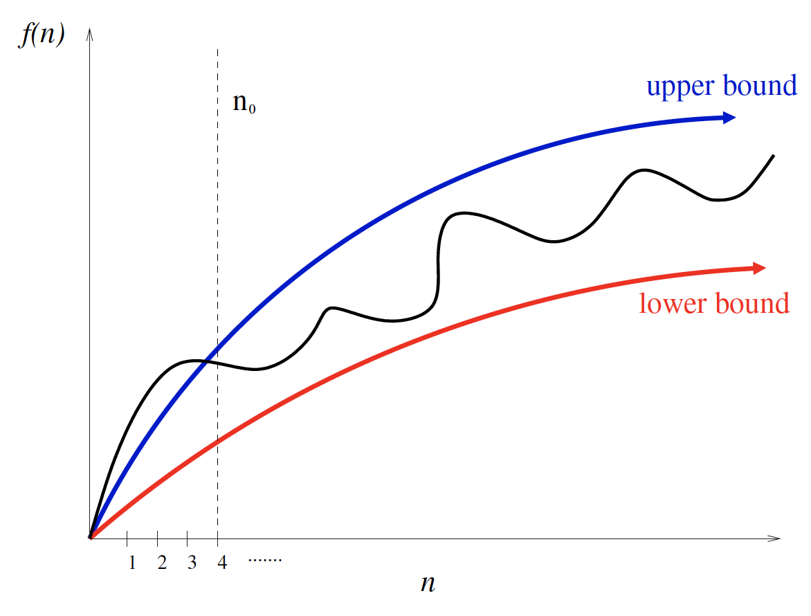
Upper and lower bounds valid for n > n0smooth out the behavior of complex functionsRequire too much detail to specify precisely — Counting the exact number of RAM instructions executed in the worst case requires the algorithm be specified to the detail of a complete computer program. Furthermore, the precise answer depends upon uninteresting coding details (e.g., did the code use a case statement or nested ifs?). Performing a precise worst-case analysis like
would clearly be very difficult work, but provides us little extra information than the observation that "the time grows quadratically with ."
It proves to be much easier to talk in terms of simple upper and lower bounds of time-complexity functions using the Big Oh notation. The Big Oh simplifies our analysis by ignoring levels of detail that do not impact our comparison of algorithms.
The Big Oh notation ignores the difference between multiplicative constants. The functions and are identical in Big Oh analysis. This makes sense given our application. Suppose a given algorithm in (say) C language ran twice as fast as one with the same algorithm written in Java. This multiplicative factor of two can tell us nothing about the algorithm itself, because both programs implement exactly the same algorithm. We should ignore such constant factors when comparing two algorithms.
The formal definitions associated with the Big Oh notation are as follows:
- Worst-case: means is an upper bound on . Thus, there exists some constant such that for every large enough (that is, for all , for some constant ).
- Best-case: means is a lower bound on . Thus, there exists some constant such that for all .
- Average-case: means is an upper bound on and is a lower bound on , for all . Thus, there exist constants and such that and for all . This means that provides a nice, tight bound on .
These definitions are illustrated below:
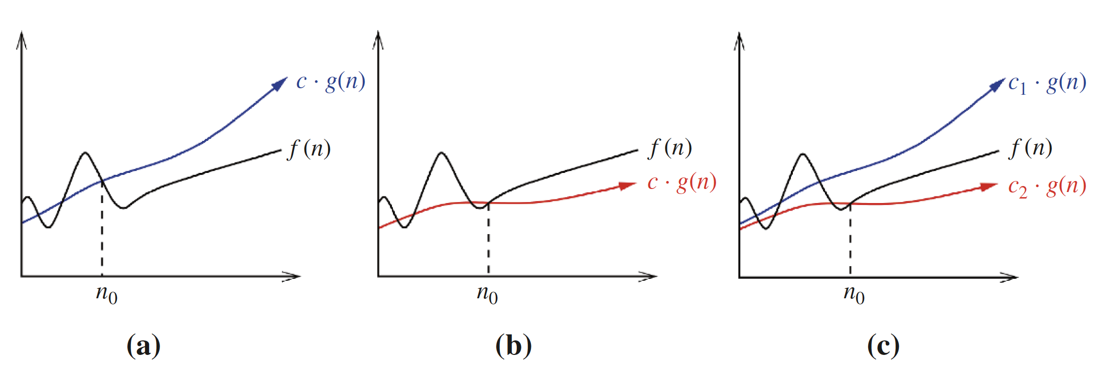
- (a):
- (b):
- (c):
Each of these definitions assumes there is a constant beyond which they are satisfied. We are not concerned about small values of , anything to the left of . After all, we don't really care whether one sorting algorithm sorts six items faster than another, but we do need to know which algorithm proves faster when sorting 10,000 or 1,000,000 items. The Big Oh notation enables us to ignore details and focus on the big picture.
| Function and complexity | Justification |
|---|---|
| Because for , . | |
| Because for , when . | |
| Because for any , when , since implies that , which implies that , which implies that . |
Growth rates and dominance relations
tbds
Working with the Big Oh
tbds
Reasoning about efficiency
tbds
Summations
tbds
Logarithms and their applications
tbds
Properties of logarithms
tbds
Advanced analysis
tbds
War story: Mystery of the pyramids
tbds
Take-home lessons
RAM model of computation
Algorithms can be understood and studied in a language- and machine-independent manner thanks to the RAM model of computation. [3]
Time complexities are well-defined functions
Each of the time complexities (i.e., best-case, worst-case, average-case) defines a numerical function for any given algorithm, representing running time as a function of input size. These functions are just as well defined as any other numerical function, be it or the price of Alphabet stock as a function of time. But time complexities are such complicated functions that we must simplify them for analysis using the "Big Oh" notation. [3]
Analyzing efficiency of algorithms
The Big Oh notation and worst-case analysis are tools that greatly simplify our ability to compare the efficiency of algorithms. [3]