Introduction to Algorithm Design

Robot tour optimization problem

Algorithm problem definition

• Problem: Robot tour optimiztion
• Input: A set $S$ of $n$ points in the plane.
• Output: What is the shortest cycle tour that visits each point in the set $S$?

Nearest neighbor heuristic

Pseudocode

% page 6 of Algorithm Design Manual
\begin{algorithm}
\caption{Nearest Neighbor Heuristic}
\begin{algorithmic}
\PROCEDURE{NearestNeighbor}{$P$}
  \STATE Pick and visit an initial point $p_0$ from $P$
  \STATE $p=p_0$
  \STATE $i=0$
  \WHILE{there are still unvisited points}
    \STATE $i=i+1$
    \STATE Select $p_i$ to be the closest unvisited point to $p_{i-1}$
    \STATE Visit $p_i$
  \ENDWHILE
  \STATE Return to $p_0$ from $p_{n-1}$
\ENDPROCEDURE
\end{algorithmic}
\end{algorithm}

Good instance

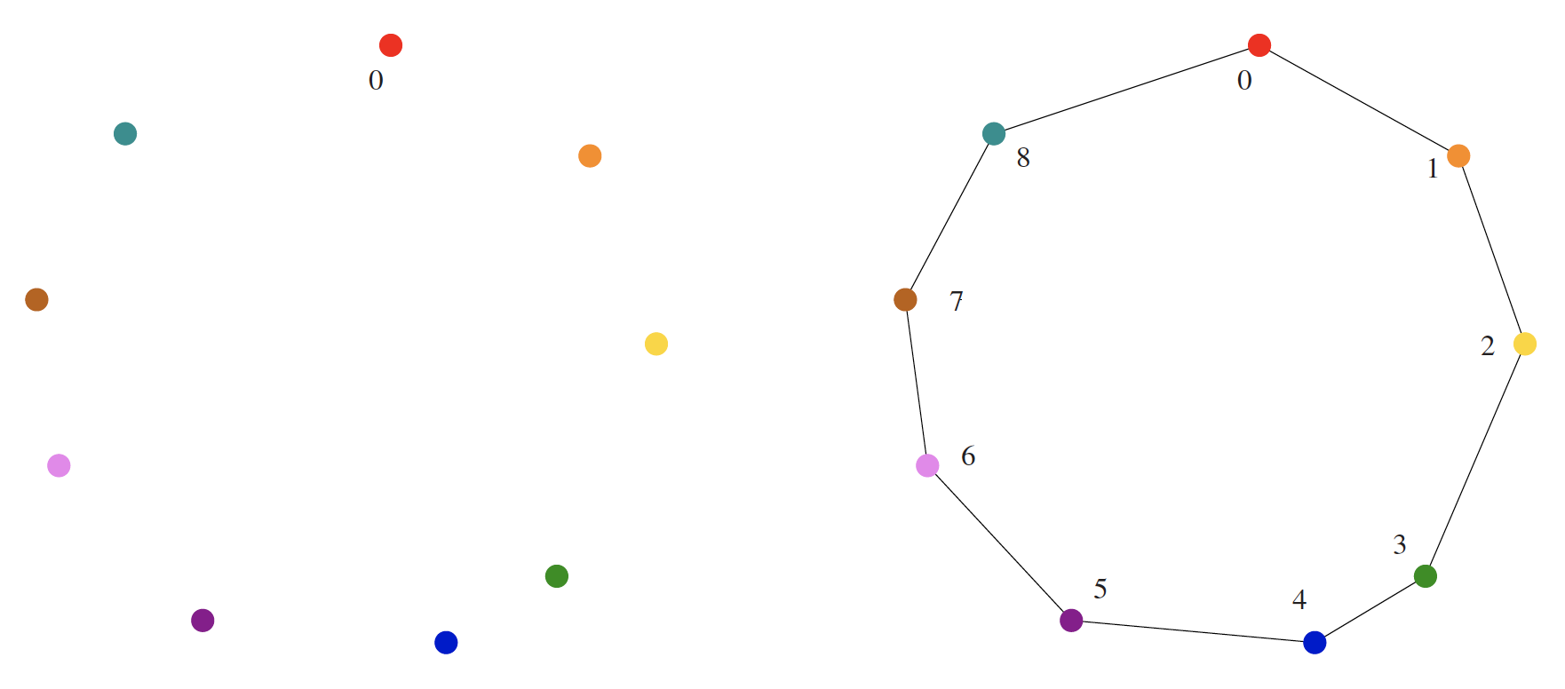
The image above shows a good instance for the nearest-neighbor heuristic. The rainbow coloring (red to violet) reflects the order of incorporation. It is clear from the images that the optimal solution is obtained as depicted. The algorithm described in pseudocode works perfectly here.

Bad instance

Top Image Coloring Error

The top image in the figure below should have its coloring reversed to reflect a rainbow sequence ordering.

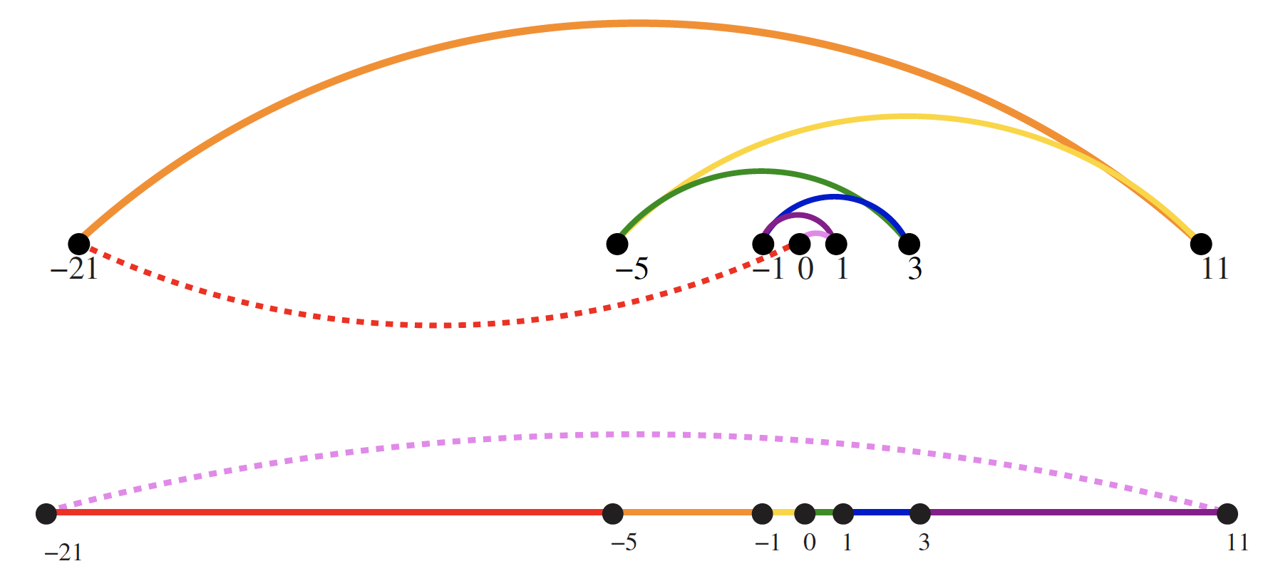
The image above depicts a bad instance for the nearest-neighbor heuristic. Specifically, consider the top figure in the image above. The numbers describe the distance that each point lies to the left or right of the point labeled 0. When we start from 0 and repeatedly walk to the nearest unvisited neighbor, we might keep jumping left–right–left–right over 0 as the algorithm offers no advice on how to break ties (keep in mind the need for the coloring to be reversed as warned above).

The distance that might be covered in such an instance is as followed (distance from one point to the next shown in blue):

$$0\stackrel{\color{blue}{1}}{\to} 1\stackrel{\color{blue}{2}}{\to} -1\stackrel{\color{blue}{4}}{\to} 3\stackrel{\color{blue}{8}}{\to} -5\stackrel{\color{blue}{16}}{\to} 11\stackrel{\color{blue}{32}}{\to} -21$$

Hence, the total distance covered in the top figure would be

$$1+2+4+8+16+32=63$$

A much better (indeed optimal) tour for these points starts from the left-most point and visits each point as we walk right before returning at the left-most point, covering a total distance of $11-(-21)=32$.

In light of our findings above, why not just start the neearest-neighbor rule using the left-most point as the initial point, $p_0$? We just showed that we can find the optimal solution in such an instance. That's true.

But what if we rotate our example by 90 degrees (clockwise or counter-clockwise)? Now all points are equally left-most. With this image in mind, imagine we pulled the 0 point out just slightly to the left. Then the 0 point is the left-most point and now instead of the robot arm jumping left-right-left-right it would be jumping up-down-up-down. The travel time will be just as bad as before.

Closest pair heuristic

Book Description

The following description is detailed in [3]:

Maybe what we need is a different approach for the instance that proved to be a bad instance for the nearest-neighbor heuristic. Always walking to the closest point is too restrictive, since that seems to trap us into making moves we didn't want.

A different idea might repeatedly connect the closest pair of endpoints whose connection will not create a problem, such as premature termination of the cycle. Each vertex begins as its own single vertex chain. After merging everything together, we will end up with a single chain containing all the points in it. Connecting the final two endpoints gives us a cycle. At any step during the execution of this closest-pair heuristic, we will have a set of single vertices and the end of vertex-disjoint chains available to merge. The pseudocode that implements this description appears below.

Pseudocode

% page 7 of Algorithm Design Manual
\begin{algorithm}
\caption{Closest Pair Heuristic}
\begin{algorithmic}
\PROCEDURE{ClosestPair}{$P$}
\STATE Let $n$ be the number of points in set $P$.
\FOR{$i=1$ to $n-1$}
  \STATE $d=\infty$
  \FOR{each pair of endpoints $(s,t)$ from distinct vertex chains}
    \IF{$\operatorname{dist}(s,t)\leq d$}
      \STATE $s_m=s$
      \STATE $t_m=t$
      \STATE $d=\operatorname{dist}(s,t)$
    \ENDIF
  \ENDFOR
  \STATE Connect $(s_m,t_m)$ by an edge
\ENDFOR
\STATE Connect the two endpoints by an edge
\ENDPROCEDURE
\end{algorithmic}
\end{algorithm}

Clarified description

The book's description of the closest pair heuristic is not as clear or easy to follow as one might hope. Consider this an attempt to add some clarity.

It may help to first "zoom back" a bit and answer the basic question of what we are trying to find in graph theory terms:

What is the shortest closed trail?

That is, we want to find a sequence of edges $(e_1,e_2,\ldots,e_{n-1})$ for which there is a sequence of vertices $(v_1,v_2,\ldots,v_n)$ where $v_1=v_n$ and all edges are distinct. The edges are weighted, where the weight for each edge is simply the distance between vertices that comprise the edge--we want to minimize the overall weight of whatever closed trails exist.

Practically speaking, the ClosestPair heuristic gives us one of these distinct edges for every iteration of the outer for loop in the pseudocode (lines 3-10), where the inner for loop (lines 5-9) ensures the distinct edge being selected at each step, $(s_m,t_m)$, is comprised of vertices coming from the endpoints of distinct vertex chains; that is, $s_m$ comes from the endpoint of one vertex chain and $t_m$ from the endpoint of another distinct vertex chain. The inner for loop simply ensures we consider all such pairs, minimizing the distance between potential vertices in the process.

Ties

One potential source of confusion is that no sort of "processing order" is specified in either for loop. How do we determine the order in which to compare endpoints and, furthermore, the vertices of those endpoints? It doesn't matter. The nature of the inner for loop makes it clear that, in the case of ties, the most recently encountered vertex pairing with minimal distance is chosen.

Good instance

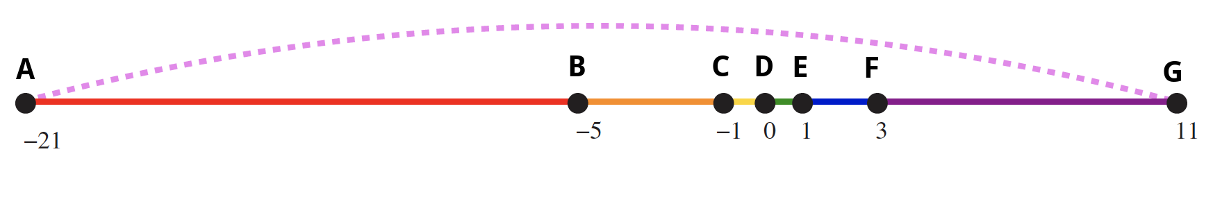
Recall what happened in the bad instance of applying the NearestNeighbor heuristic (observe the newly added vertex labels):

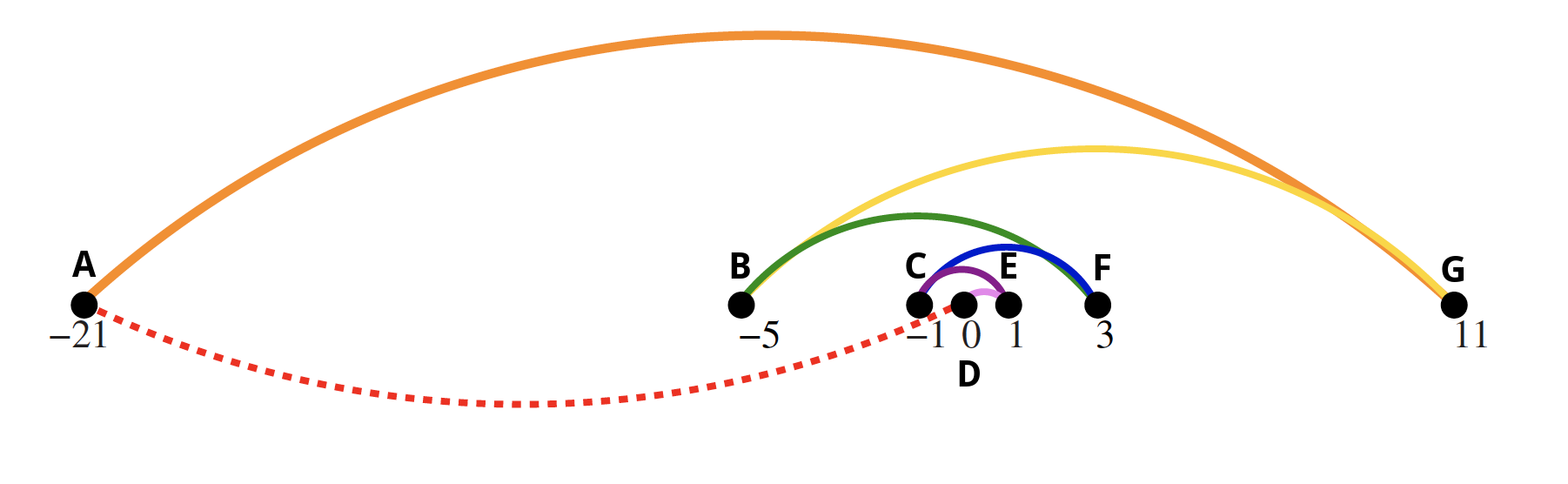
The total distance covered was absurd because we kept jumping back and forth over 0.

Now consider what happens when we use the ClosestPair heuristic. We have $n=7$ vertices; hence, the pseudocode indicates that the outer for loop will be executed 6 times. As the book notes, each vertex begins as its own single vertex chain (i.e., each point is a singleton where a singleton is a chain with one endpoint). In our case, given the figure above, how many times will the inner for loop execute? Well, how many ways are there to choose a 2-element subset of an $n$-element set (i.e., the 2-element subsets represent potential vertex pairings)? There are $n$ choose 2 such subsets:

$$\binom{n}{2}=\frac{n!}{2!(n-2)!}=\frac{n(n-1)}{2}$$

Since $n=7$ in our case, there's a total of 21 possible vertex pairings to investigate. The nature of the figure above makes it clear that (C, D) and (D, E) are the only possible outcomes from the first iteration since the smallest possible distance between vertices in the beginning is 1 and $\dist(C, D)=\dist(D, E)=1$. Which vertices are actually connected to give the first edge, (C, D) or (D, E), is unclear since there is no processing order. Let's assume we encounter vertices D and E last, thus resulting in (D, E) as our first edge.

Now there are 5 more iterations to go and 6 vertex chains to consider: A, B, C, (D, E), F, G.

Each Iteration Eliminates a Vertex Chain

Each iteration of the outer for loop in the ClosestPair heuristic results in the elimination of a vertex chain. The outer for loop iterations continue until we are left with a single vertex chain comprised of all vertices, where the last step is to connect the two endpoints of this single vertex chain by an edge.

More precisely, for a graph $G$ comprised of $n$ vertices, we start with $n$ vertex chains (i.e., each vertex begins as its own single vertex chain). Each iteration of the outer for loop results in connecting two vertices of $G$ in such a way that these vertices come from distinct vertex chains; that is, connecting these vertices results in merging two distinct vertex chains into one, thus decrementing by 1 the total number of vertex chains left to consider.

Repeating such a process $n-1$ times for a graph that has $n$ vertices results in being left with $n-(n-1)=1$ vertex chain, a single chain containing all the points of $G$ in it. Connecting the final two endpoints gives us a cycle.

One possible depiction of how each iteration looks is as follows:

ClosestPair outer for loop iterations
  1: connect D to E # -> dist: 1, chains left (6): A, B, C, (D, E), F, G
  2: connect D to C # -> dist: 1, chains left (5): A, B, (C, D, E), F, G
  3: connect E to F # -> dist: 3, chains left (4): A, B, (C, D, E, F), G
  4: connect C to B # -> dist: 4, chains left (3): A, (B, C, D, E, F), G
  5: connect F to G # -> dist: 8, chains left (2): A, (B, C, D, E, F, G)
  6: connect B to A # -> dist: 16, single chain: (A, B, C, D, E, F, G)

Final step: connect A and G

Hence, the ClosestPair heuristic does the right thing in this example where previously the NearestNeighbor heuristic did the wrong thing:

But not on all examples.

Bad instance

Consider what the ClosestPair algorithm does on the point set in the figure below (it may help to first try imagining the point set without any edges connecting the vertices):

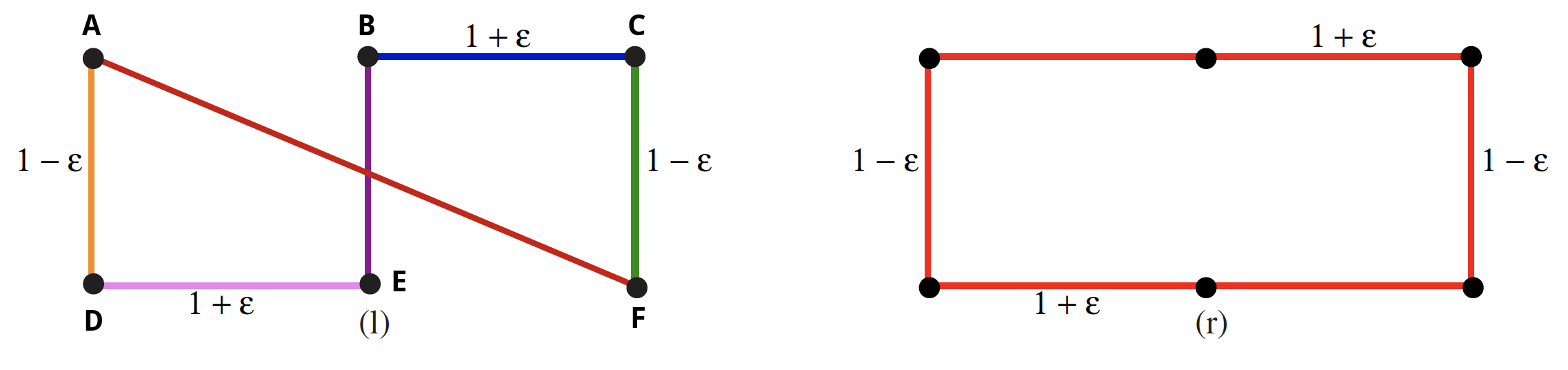
How can we connect the vertices using ClosestPair? We have $n=6$ vertices; thus, the outer for loop will execute $6-1=5$ times, where our first order of business is to investigate the distance between vertices of

$$\binom{6}{2}=\frac{6!}{2!(6-2)!}=\frac{6\cdot 5}{2}=15$$

total possible pairs. The figure above helps us see that $\dist(A,D)=\dist(B,E)=\dist(C,F)=1-\varepsilon$ are the only possible options in the first iteration since $1-\varepsilon$ is the shortest distance between any two vertices. We arbitrarily choose (A, D) as the first pairing.

Now are there are 4 more iterations to go and 5 vertex chains to consider: (A, D), B, C, E, F. One possible depiction of how each iteration looks is as follows:

ClosestPair outer for loop iterations
  1: connect A to D # --> dist: 1-ɛ, chains left (5): (A, D), B, C, E, F
  2: connect B to E # --> dist: 1-ɛ, chains left (4): (A, D), (B, E), C, F
  3: connect C to F # --> dist: 1-ɛ, chains left (3): (A, D), (B, E), (C, F)
  4: connect D to E # --> dist: 1+ɛ, chains left (2): (A, D, E, B), (C, F)
  5: connect B to C # --> dist: 1+ɛ, single chain: (A, D, E, B, C, F)

Final step: connect A and F

Correctly Considering the Endpoints to Connect from Distinct Vertex Chains

Iterations 1-3 depicted above are fairly uneventful in the sense that we have no other meaningful options to consider. Even once we have the distinct vertex chains (A, D), (B, E), and (C, F), the next choice is similarly uneventful and arbitrary. There are four possibilities given that the smallest possible distance between vertices on the fourth iteration is $1+\varepsilon$:

(A, B), (D, E), (B, C), (E, F)

The distance between vertices for all of the points above is $1+\varepsilon$. The choice of (D, E) is arbitrary. Any of the other three vertex pairings would have worked just as well. But notice what happens during iteration 5--our possible choices for vertex pairings have been tightly narrowed.

Specifically, the vertex chains (A, D, E, B) and (C, F), which have endpoints (A, B) and (C, F), respectively, allow for only four possible vertex pairings:

(A, C), (A, F), (B, C), (B, F)

Even if it may seem obvious, it is worth explicitly noting that neither D nor E were viable vertex candidates above--neither vertex is included in the endpoint, (A, B), of the vertex chain of which they are vertices, namely (A, D, E, B).

There is no arbitrary choice at this stage. There are no ties in the distance between vertices in the pairs above. The (B, C) pairing results in the smallest distance between vertices: $1+\varepsilon$. Once vertices B and C have been connected by an edge, all iterations have been completed and we are left with a single vertex chain: (A, D, E, B, C, F). Connecting A and F gives us a cycle and concludes the process.

The total distance traveled across (A, D, E, B, C, F) is as follows:

$$\underbrace{(1-\varepsilon)}_{\texttt{A}\to\texttt{D}} + \underbrace{(1+\varepsilon)}_{\texttt{D}\to\texttt{E}} + \underbrace{(1-\varepsilon)}_{\texttt{E}\to\texttt{B}} + \underbrace{(1+\varepsilon)}_{\texttt{B}\to\texttt{C}} + \underbrace{(1-\varepsilon)}_{\texttt{C}\to\texttt{F}} + \underbrace{\sqrt{(1-\varepsilon)^2+(2+2\varepsilon)^2}}_{\texttt{F}\to\texttt{A}}$$

The distance above evaluates to

$$5-\epsilon+\sqrt{5\varepsilon^2+6\varepsilon+5}$$

as opposed to the total distance traveled by just going around the boundary (the right-hand figure in the image above where all edges are colored in red): $6+2\varepsilon$.

As $\varepsilon\to0$, we see that

$$5+\sqrt{5}\approx7.24 > 6,$$

where 6 units was the necessary amount of travel. Hence, we end up traveling about

$$\frac{(5+\sqrt{5})-6}{6}\times 100\approx 20.6\%$$

farther than is necessary by using the ClosestPair heuristic in this case. As noted in [3], examples exist where the penalty is considerably worse than this.

Enumerate all possibilities

Given the issues encountered when trying to use the nearest neighbor and closest pair heuristics, we could try enumerating all possible orderings of the set of points and then select the one that minimizes the total length:

% page 8 of Algorithm Design Manual
\begin{algorithm}
\caption{Optimal Traveling Salesman Problem (TSP)}
\begin{algorithmic}
\PROCEDURE{OptimalTSP}{$P$}
\STATE $d=\infty$
\FOR{each of the $n!$ permutations $P_i$ of point set $P$}
  \IF{$\operatorname{cost}(P_i)\leq d$}
    \STATE $d=\operatorname{cost}(P_i)$
    \STATE $P_{\min} = P_i$
  \ENDIF
\ENDFOR
\RETURN $P_{\min}$
\ENDPROCEDURE
\end{algorithmic}
\end{algorithm}

Since all possible orderings are considered, we are guaranteed to end up with the shortest possible tour. This algorithm is correct, since we pick the best of all the possibilities. But it is also extremely slow. Even a powerful computer couldn't hope to enumerate all the 20! = 2,432,902,008,176,640,000 orderings of 20 points within a day. For real circuit boards, where n ≈ 1,000, forget about it. All of the world's computers working full time wouldn't come close to finishing the problem before the end of the universe, at which point it presumably becomes moot.

The quest for an efficient algorithm to solve this problem, called the traveling salesman problem (TSP), will take us through much of this book.

Movie scheduling problem

Consider the following scheduling problem. Imagine you are a highly in demand actor, who has been presented with offers to star in $n$ different movie projects under development. Each offer comes specified with the first and last day of filming. Whenever you accept a job, you must commit to being available throughout this entire period. Thus, you cannot accept two jobs whose intervals overlap.

For an artist such as yourself, the criterion for job acceptance is clear: you want to make as much money as possible. Because each film pays the same fee, this implies you seek the largest possible set of jobs (intervals) such that no two of them conflict with each other.

For example, an optimal solution to this problem is highlighted in red below:

Algorithm problem definition

• Problem: Movie scheduling problem
• Input: A set $I$ of $n$ intervals on the line.
• Output: What is the largest subset of mutually non-overlapping intervals that can be selected from $I$?

Earliest job first

There are several ideas that may come to mind. One is based on the notion that it is best to work whenever work is available. This implies that you should start with the job with the earliest start date:

% page 8 of Algorithm Design Manual
\begin{algorithm}
\caption{Earliest Job First}
\begin{algorithmic}
\PROCEDURE{EarliestJobFirst}{$I$}
\STATE Accept the earliest starting job $j$ from $I$ that does not overlap any previously accepted job.
\STATE Repeat until no more such jobs remain.
\ENDPROCEDURE
\end{algorithmic}
\end{algorithm}

This idea makes sense, at least until we realize that accepting the earliest job might block us from taking many other jobs if that first job is long:

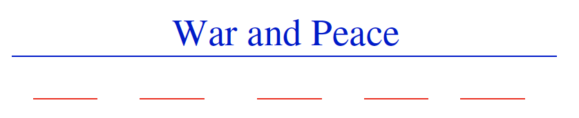
Above, we see that War and Peace, the job with the earliest start date, prevents us from getting work for four other jobs (the optimal solution in red).

All Jobs Pay the Same (flat fee)

Remember that one of the conditions of the problem is that all jobs pay the same. So you're wanting to maximize the total overall number of jobs you can get.

Shortest job first

Given the flat fee nature of payments for different jobs, maybe we would be better off selecting the shortest job first and proceed to eliminate other overlapping jobs:

% page 8 of Algorithm Design Manual
\begin{algorithm}
\caption{Shortest Job First}
\begin{algorithmic}
\PROCEDURE{ShortestJobFirst}{$I$}
\WHILE{$I\neq\emptyset$}
  \STATE Accept the shortest possible job $j$ from $I$.
  \STATE Delete $j$, and any interval that intersects $j$, from $I$.
\ENDWHILE
\ENDPROCEDURE
\end{algorithmic}
\end{algorithm}

As with the "earliest job first" approach, this idea makes sense at first. At least until we realize that accepting the shortest job might block us from taking two other jobs:

Exhaustive scheduling

This problem is starting to feel like the robot tour optimization problem. Should we ditch attempts at clever approaches and go for enumerating all scheduling possibilities and select the best result?

We can try (pseudocode below ignores the details of testing whether or not a set of intervals is, in fact, disjoint):

% page 8 of Algorithm Design Manual
\begin{algorithm}
\caption{Exhaustive Scheduling}
\begin{algorithmic}
\PROCEDURE{ExhaustiveScheduling}{$I$}
\STATE $j=0$
\STATE $S_{\max}=\emptyset$
\FOR{each of the $2^n$ subsets $S_i$ of intervals $I$}
  \IF{($S_i$ is mutually non-overlapping) and ($\operatorname{size}(S_i)>j$)}
    \STATE $j=\operatorname{size}(S_i)$
    \STATE $S_{\max}=S_i$
  \ENDIF
\ENDFOR
\RETURN $S_{\max}$
\ENDPROCEDURE
\end{algorithmic}
\end{algorithm}

Is the slowness of this approach prohibitive like the exhaustive approach was for the robot tour optimization problem? The critical limitation is enumerating the $2^n$ subsets of $n$ things. Enumerating $2^n$ items is much better than enumerating $n!$ items. For smaller $n$-values, like say $n=20$, we get about a million subsets. But for something like $n=100$, we get $2^{100}$, which is much greater than any set of computers could hope to enumerate.

Earliest terminating job first (optimal scheduling)

Spoiler alert: The difference between our scheduling and robotics problems is that there is an algorithm that solves the movie scheduling both correctly and efficiently.

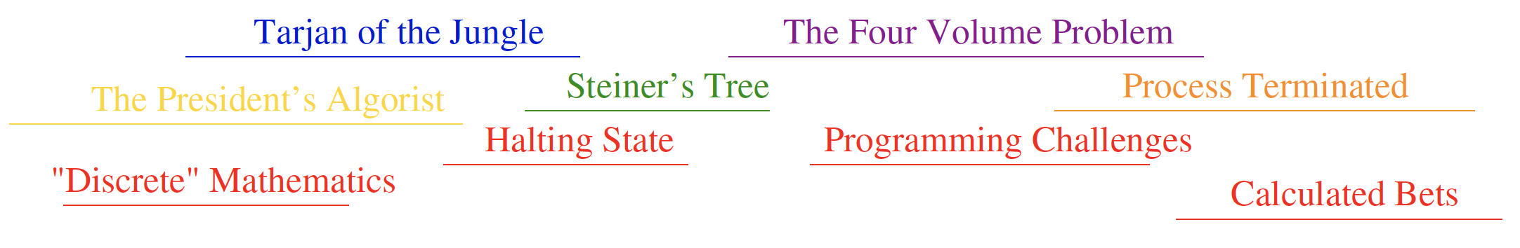
Think about the first job to terminate; that is, the interval $x$ whose right endpoint is left-most among all intervals. This role is played by "Discrete" Mathematics in the figure below:

Other jobs may well have started before $x$ (e.g., The President's Algorist), but all of these must at least partially overlap each other (otherwise the right endpoint of $x$ would not represent the earliest termination date for a set of jobs). Thus, we can select at most one job from the group. The first of these jobs to terminate is $x$, so any of the overlapping jobs potentially block out other opportunities to the right of it. Clearly we can never lose by picking $x$. This suggests the following correct, efficient algorithm:

% page 8 of Algorithm Design Manual
\begin{algorithm}
\caption{Optimal Scheduling}
\begin{algorithmic}
\PROCEDURE{OptimalScheduling}{$I$}
\WHILE{$I\neq\emptyset$}
  \STATE Accept the job $j$ from $I$ with the earliest completion date.
  \STATE Delete $j$, and any interval which intersects $j$, from $I$.
\ENDWHILE
\ENDPROCEDURE
\end{algorithmic}
\end{algorithm}

In the figure above, this process looks as follows:

Pick -> "Discrete" Mathematics
  Eliminate -> The President's Algorist, Tarjan of the Jungle
Pick -> Halting State
  Eliminate -> Steiner's Tree
Pick -> Programming Challenges
  Eliminate -> The Four Volume Problem, Process Terminated
Pick -> Calculated Bets

Counterexamples

Two important properties

Verifiability

To demonstrate that a particular instance is a counterexample to a particular algorithm, you must be able to

1. calculate what answer your algorithm will give in this instance, and
2. display a better answer so as to prove that the algorithm didn't find it.

Simplicity

Good counter-examples have all unnecessary details stripped away. They make clear exactly why the proposed algorithm fails. Simplicity is important because you must be able to hold the given instance in your head in order to reason about it. Once a counterexample has been found, it is worth simplifying it down to its essence.

Techniques

Hunting for counterexamples is a skill worth developing. It bears some similarity to the task of developing test sets for computer programs, but relies more on inspiration than exhaustion. Here are some techniques to aid your quest:

Think small

Note that the robot tour counter-examples I presented boiled down to only considering a few points, and the scheduling counter-examples to only a few intervals. This is indicative of the fact that when algorithms fail, there is usually a very simple example on which they fail. Amateur algorists tend to draw a big messy instance and then stare at it helplessly. The pros look carefully at several small examples, because they are easier to verify and reason about.

Think exhaustively

There are usually only a small number of possible instances for the first non-trivial value of $n$. For example, there are only three distinct ways two intervals on the line can occur:

• as disjoint intervals
• as overlapping intervals
• as properly nesting intervals, one within the other

All cases of three intervals (including counter-examples to both of the movie heuristics) can be systematically constructed by adding a third segment in each possible way to these three instances.

Hunt for the weakness

If a proposed algorithm is of the form "always take the biggest" (better known as the greedy algorithm), think about why that might prove to be the wrong thing to do. In particular, go for a tie.

Go for a tie

A devious way to break a greedy heuristic is to provide instances where everything is the same size. Suddenly the heuristic has nothing to base its decision on, and perhaps has the freedom to return something suboptimal as the answer.

For example, recall the issues we encountered when we tried to employ the nearest neighbor heuristic to optimize the robot's tour. Since distances were the same at different points, with no decision-making criteria other than a greedy approach, this led to a variety of different issues.

Seek extremes

Many counter-examples are mixtures of huge and tiny, left and right, few and many, near and far. It is usually easier to verify or reason about extreme examples than more muddled ones. Consider two tightly bunched clouds of points separated by a much larger distance $d$. The optimal TSP tour will be essentially $2d$ regardless of the number of points, because what happens within each cloud doesn't really matter.

Greedy movie stars

Problem

Recall the movie star scheduling problem, where we seek to find the largest possible set of non-overlapping intervals in a given set $S$. A natural greedy heuristic selects the interval $i$, which overlaps the smallest number of other intervals in $S$, removes them, and repeats until no intervals remain.

Give a counter-example to this proposed algorithm.

Solution

Consider the following figure:

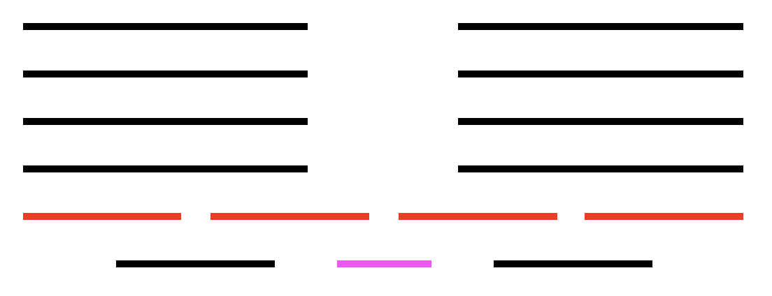
Removing the job colored in pink results in removing the two jobs colored in red above it. But those two jobs are part of the optimal solution colored in red (all other solutions result in only being able to choose 3 jobs instead of the 4 pictured in red).

Constructing the counterexample

The counterexample above is nice, but how does one go about constructing something like that? Skiena's thought process, as detailed in [3], was as follows:

• Start with an odd-length chain of intervals, each of which overlaps one interval to the left and one to the right. Picking an even-length chain would mess up the optimal solution (hunt for the weakness).
• All intervals overlap two others, except for the left and right-most intervals (go for the tie).
• To make these terminal intervals unattractive, we can pile other intervals on top of them (seek extremes)
• The length of our chain (7) is the shortest that permits this construction to work (aim for simplicity).

Order of Counterexample Construction

Observe that the notes above concerning the counterexample's construction occur with a bottom-up kind of ordering. That is, the odd-length chain of intervals starts at the bottom in the figure (i.e., the bottom row with black, pink, and black intervals). We ensure that each of these intervals overlaps one interval to the left and one to the right (i.e., this leads to the construction of the read intervals directly above the bottom row).

Now, all intervals so far in the construction process look as follows:

That is, all intervals overlap two others, except for the left- and right-most intervals. To make these terminal intervals unattractive, we pile other intervals on top of them (this leads to the complete figure with the piled on intervals in black above those in red).

With the complete picture in hand, we can see that any black interval in any of the top four rows overlaps 6 other intervals (i.e., 3 other black intervals above or below the one selected in the top four rows, 2 red intervals below it, and the black interval below the red intervals). Each red interval overlaps 5 black intervals. Each black interval on the bottom overlaps 6 intervals (the 2 red intervals immediately above and then the 4 black intervals above them).

We are finally left with the pink interval which overlaps the smallest number of other intervals, namely 2 (i.e., the 2 red intervals directly above it). The chain link of 7 Skiena refers to is in reference to the number of intervals in the figure above before the other intervals are piled on.

Induction and recursion

Recursion is mathematical induction in action. In both, we have general and boundary conditions, with the general condition breaking the problem into smaller and smaller pieces. The initial or boundary condition terminates the recursion.

Once you understand either recursion or induction, you should be able to see why the other one also works.

Incremental correctness

Consider the following algorithm:

% page 8 of Algorithm Design Manual
\begin{algorithm}
\caption{Recursive Algorithm for Incrementing Natural Numbers}
\begin{algorithmic}
\PROCEDURE{Incremenet}{$y$}
\IF{$y=0$}
  \RETURN 1
\ELSE
  \IF{$y\bmod 2 = 1$}
    \RETURN $2\,\cdot$ \CALL{Increment}{$\lfloor y/2\rfloor$}
  \ELSE
    \RETURN $y+1$
  \ENDIF
\ENDIF
\ENDPROCEDURE
\end{algorithmic}
\end{algorithm}

Prove the correctness of this recursive algorithm for incrementing natural numbers by proving that $\operatorname{Increment}(y)$ returns $y+1$ for all natural numbers $y$, where "natural numbers" refers to the set of non-negative integers.

Working out the solution to this problem implicitly requires us to know the difference between weak and strong induction as well as how to write an induction proof.

Let's illustrate how to do both by first starting out with an explicit problem statement.

Problem: Prove that $\operatorname{Increment}(y)\to y+1$ holds for all $y\geq0$.

Solution: For any integer $y\geq0$, let $S(y)$ denote the statement

$$S(y)\colon \operatorname{Increment}(y)\to y+1$$

Base step ($y=0$): $S(0)$ says that $\operatorname{Increment}(0)\to 0+1=1$, which is trivially true due to lines 2-3 of the pseudocode spelled out for the Increment method (i.e., $\operatorname{Increment}(0)$ returns 1 if $y=0$, as it does for the base case).

Inductive step [$S(k)\to S(k+1)$]: Fix some $k\geq0$, and assume that for every $t$ satisfying $0\leq t\leq k$, the statement $S(t)$ is true. To be shown is that

$$S(k+1)\colon \operatorname{Increment}(k+1)\to (k+1)+1=k+2$$

follows. Let's start by considering what happens when $k+1$ is even. Then $(k+1)\bmod 2 = 0$ resulting in $\operatorname{Increment}(k+1)\to(k+1)+1=k+2$, as desired. But what if $k+1$ is odd? Then $k+1=2\ell+1$ where $\ell\in\Z$ (note that this implies $0\leq\ell\leq k$), and

$$(k+1)\bmod 2 = (2\ell+1)\bmod 2 = 1$$

which means we have the following:

$$\begin{align*} \operatorname{Increment}(k+1) &\to 2\cdot\operatorname{Increment}(\lfloor (k+1)/2\rfloor) & \text{(since $(k+1)\bmod 2 = 1$)}\\[0.5em] &= 2\cdot\operatorname{Increment}(\lfloor (2\ell+1)/2\rfloor) & \text{(since $k+1=2\ell+1$)}\\[0.5em] &= 2\cdot\operatorname{Increment}(\ell) & \text{(since $\lfloor (2\ell+1)/2\rfloor=\lfloor \ell+\frac{1}{2} \rfloor=\ell$)}\\[0.5em] &= 2\cdot(\ell+1) & \text{(by $S(k)$, the ind. hyp.)}\\[0.5em] &= (2\ell+1)+1\\[0.5em] &= (k+1)+1\\[0.5em] &= k+2 \end{align*}$$

Need for Strong Induction

Note that the argument above requires the use of strong induction since Increment may be assumed to work by the inductive hypothesis for $y = k$ but not for a value that is about half of it (i.e., $\lfloor k/2\rfloor$).

The reason we are allowed to assume that $\operatorname{Increment}(\ell)\to\ell+1$ in the argument above is due to the fact that we fixed some $k\geq0$ and assumed that $S(k)$ held for every $t$ satisfying $0\leq t\leq k$ (the inductive hypothesis). When we set $k+1=2\ell+1$, where $\ell\in\Z$, we can easily see that $k=2\ell$, which means $\ell\in[0,k]$, indicating the inductive hypothesis may be applied to $\ell$ (i.e., $S(\ell)$) since the inductive hypothesis may be applied to all $t$ for which $0\leq t\leq k$.

Modeling the problem

Modeling is the art of formulating your application in terms of precisely described, well-understood problems. Proper modeling is the key to applying algorithmic design techniques to real-world problems. Real-world applications involve real-world objects. You might be working on a system to route traffic in a network, to find the best way to schedule classrooms in a university, or to search for patterns in a corporate database. Most algorithms, however, are designed to work on rigorously defined abstract structures such as permutations, graphs, and sets. To exploit the algorithms literature, you must learn to describe your problem abstractly, in terms of procedures on such fundamental structures.

Combinatorial objects

Odds are very good that others have probably stumbled upon any algorithmic problem you care about, perhaps in substantially different contexts. But to find out what is known about your particular "widget optimization problem," you can't hope to find it in a book under widget. You must first formulate widget optimization in terms of computing properties of common structures such as those described below.

Permutations

Permutations are arrangements, or orderings, of items. For example, $\{1,4,3,2\}$ and $\{4,3,2,1\}$ are two distinct permutations of the same set of four integers. We have already seen permutations in the robot optimization problem, and in sorting.

Permutations are likely the object in question whenever your problem seeks an "arrangement," "tour," "ordering," or "sequence."

Subsets

Subsets represent selections from a set of items. For example, $\{1,3,4\}$ and $\{2\}$ are two distinct subsets of the first four integers. Order does not matter in subsets the way it does with permutations, so the subsets $\{1,3,4\}$ and $\{4,3,1\}$ would be considered identical. Subsets arose as candidate solutions in the movie scheduling problem.

Subsets are likely the object in question whenever your problem seeks a "cluster," "collection," "committee," "group," "packaging," or "selection."

Trees

Trees represent hierarchical relationships between items.

Trees are likely the object in question whenever your problem seeks a "hierarchy," "dominance relationship," "ancestor/descendant relationship," or "taxonomy."

Graphs

Graphs represent relationships between arbitrary pairs of objects.

Graphs are likely the object in question whenever you seek a "network," "circuit," "web," or "relationship."

Points

Points define locations in some geometric space. For example, the locations of McDonald's restaurants can be described by points on a map/plane.

Points are likely the object in question whenever your problems work on "sites," "positions," "data records," or "locations."

Polygons

Polygons define regions in some geometric spaces. For example, the borders of a country can be described by a polygon on a map/plane.

Polygons and polyhedra are likely the object in question whenever you are working on "shapes," "regions," "configurations," or "boundaries."

Strings

Strings represent sequences of characters, or patterns. For example, the names of students in a class can be represented by strings.

Strings are likely the object in question whenever you are dealing with "text," "characters," "patterns," or "labels."

Use the Language of Fundamental Structures to Describe Application Models

The fundamental structures/combinatorial objects mentioned above all have associated algorithm problems, which are presented in the catalog. Familiarity with these problems is important, because they provide the language we use to model applications. To become fluent in this vocabulary, browse through the catalog and study the input and output pictures for each problem. Understanding these problems, even at a cartoon/definition level, will enable you to know where to look later when the problem arises in your application.

Modeling is only the first step in designing an algorithm for a problem. Be alert for how the details of your applications differ from a candidate model, but don't be too quick to say that your problem is unique and special. Temporarily ignoring details that don't fit can free the mind to ask whether they really were fundamental in the first place.

Always try to model your application in terms of standard algorithm problems. You can then use the catalog to pull out what is known about any given problem whenever it is needed.

Recursive objects

Learning to think recursively is learning to look for big things that are made from smaller things of exactly the same type as the big thing. If you think of houses as sets of rooms, then adding or deleting a room still leaves a house behind. Recursive structures occur everywhere in the algorithmic world. Indeed, each of the abstract combinatorial objects described above can be thought about recursively. You just have to see how you can break them down:

Recursive decompositions of combinatorial objects. Permutations, subsets, trees, and graphs (left column). Point sets, polygons, and strings (right column).

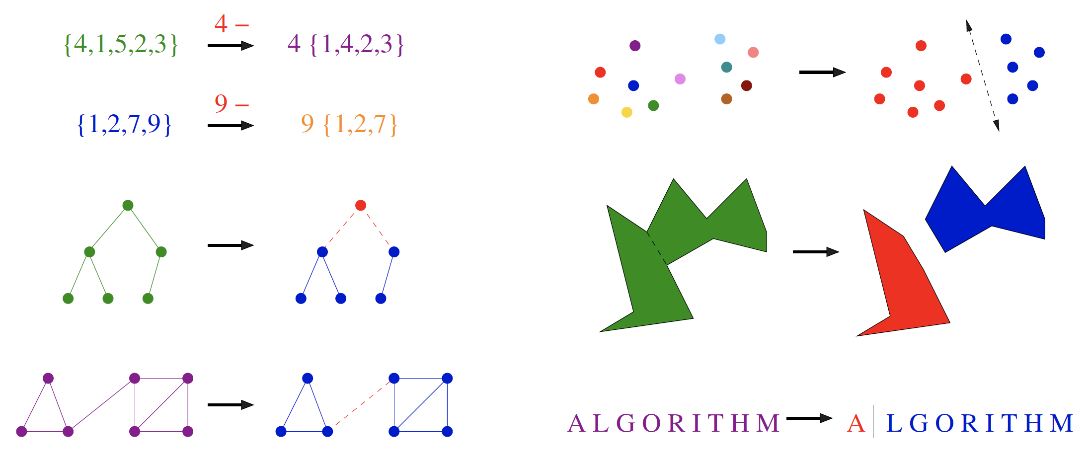
Permutations

Delete the first element of a permutation of $n$ things $\{1, . . . , n\}$ and you get a permutation of the remaining $n−1$ things. This may require renumbering to keep the object a permutation of consecutive integers. For example, removing the first element of $\{4,1,5,2,3\}$ and renumbering gives $\{1,4,2,3\}$, a permutation of $\{1,2,3,4\}$. Permutations are recursive objects.

Subsets

Every subset of $\{1,\ldots,n\}$ contains a subset of $\{1,\ldots,n−1\}$ obtained by deleting element $n$, if it is present. Subsets are recursive objects.

Trees

Delete the root of a tree and what do you get? A collection of smaller trees. Delete any leaf of a tree and what do you get? A slightly smaller tree. Trees are recursive objects.

Graphs

Delete any vertex from a graph, and you get a smaller graph. Now divide the vertices of a graph into two groups, left and right. Cut through all edges that span from left to right, and what do you get? Two smaller graphs, and a bunch of broken edges. Graphs are recursive objects.

Points

Take a cloud of points, and separate them into two groups by drawing a line. Now you have two smaller clouds of points. Point sets are recursive objects.

Polygons

Inserting any internal chord between two non-adjacent vertices of a simple polygon cuts it into two smaller polygons. Polygons are recursive objects.

Strings

Delete the first character from a string, and what do you get? A shorter string. Strings are recursive objects.

Recursive Descriptions

Recursive descriptions of objects require both decomposition rules and basis cases, namely the specification of the smallest and simplest objects where the decomposition stops. These basis cases are usually easily defined. Permutations and subsets of zero things presumably look like $\{\}$. The smallest interesting tree or graph consists of a single vertex, while the smallest interesting point cloud consists of a single point. Polygons are a little trickier; the smallest genuine simple polygon is a triangle. Finally, the empty string has zero characters in it. The decision of whether the basis case contains zero or one element is more a question of taste and convenience than any fundamental principle.

War Story: Psychic Modeling

Background

The complete war story about psychic modeling can be found in [3]. For reference, this is what the President of Lotto Systems Group had to say to Skiena (roughly):

President: At Lotto Systems Group, we market a program designed to improve our customers' psychic ability to predict winning lottery numbers. In a standard lottery, each ticket consists of six numbers selected from, say, 1 to 44. However, after proper training, our clients can visualize (say) fifteen numbers out of the 44 and be certain that at least four of them will be on the winning ticket

Our problem is this. After the psychic has narrowed the choices down to fifteen numbers and is certain that at least four of them will be on the winning ticket, we must find the most efficient way to exploit this information. Suppose a cash prize is awarded whenever you pick at least three of the correct numbers on your ticket. We need an algorithm to construct the smallest set of tickets that we must buy in order to guarantee that we win at least one prize.

Skiena: Assuming the psychic is correct?

President: Yes, assuming the psychic is correct. We need a program that prints out a list of all the tickets that the psychic should buy in order to minimize their investment.

Six Numbers Chosen are Presumably Distinct

As noted in the Wiki article on lottery mathematics, a typical game involves each player choosing six distinct numbers from a given range.

Identifying the best subset of tickets to buy was very much a combinatorial algorithm problem. It was going to be some type of covering problem, where each ticket bought would "cover" some of the possible 4-element subsets of the psychic's set. Finding the absolute smallest set of tickets to cover everything was a special instance of the NP-complete problem set cover (see the catalog entry on set cover), and presumably computationally intractable.

It was indeed a special instance of set cover, completely specified by only four numbers:

• $n$: the size $n$ of the candidate set $S$ (typically $n\approx 15$),
• $k$: the number of slots $k$ for numbers on each ticket (typically $k\approx 6$),
• $j$: the number of psychically promised correct numbers $j$ from $S$ (say $j = 4$), and finally,
• $\ell$: the number of matching numbers $\ell$ necessary to win a prize (say $\ell = 3$).

The figure below illustrates a covering of a smaller instance, where $n = 5$, $k = 3$, and $\ell = 2$, and no psychic contribution (meaning $j = 5$):

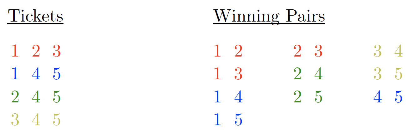
This figure represents a covering of all pairs of $\{1,2,3,4,5\}$ with tickets $\{1,2,3\}$, $\{1,4,5\}$, $\{2,4,5\}$, $\{3,4,5\}$. Pair color reflects the covering ticket.

Skiena indicates that after modeling the problem in terms of sets and subsets, the basic components of a solution seemed fairly straightforward:

• We needed the ability to generate all subsets of $k$ numbers from the candidate set $S$. Algorithms for generating and ranking/unranking subsets of sets are presented in the catalog.
• We needed the right formulation of what it meant to have a covering set of purchased tickets. The obvious criteria would be to pick a small set of tickets such that we have purchased at least one ticket containing each of the $\binom{n}{\ell}$-subsets of $S$ that might pay off with the prize.
• We needed to keep track of which prize combinations we have thus far covered. We seek tickets to cover as many thus-far-uncovered prize combinations as possible. The currently covered combinations are a subset of all possible combinations. Data structures for subsets are discussed in the catalog. The best candidate seemed to be a bit vector, which would answer in constant time "is this combination already covered?"
• We needed a search mechanism to decide which ticket to buy next. For small enough set sizes, we could do an exhaustive search over all possible subsets of tickets and pick the smallest one. For larger problems, a randomized search process like simulated annealing would select tickets-to-buy to cover as many uncovered combinations as possible. By repeating this randomized procedure several times and picking the best solution, we would be likely to come up with a good set of tickets.

After an alleged solution was found and reported to Lotto's president, the president complained the proposed number of tickets to buy was too high. Something wasn't right with whatever algorithm was used to generate the ticket purchase recommendations.

Correction

Skiena noted that the president was correct and that he and his student hadn't modeled the problem correctly. They did not need to explicitly cover all possible winning combinations. The following figure illustrates the principle by giving a two-ticket solution, namely

$$\{1,2,3\},\quad\{1,4,5\}$$

to the previous example, which involved a four-ticket solution, namely

$$\{1,2,3\},\quad\{1,4,5\},\quad\{2,4,5\},\quad\{3,4,5\}$$

The figure

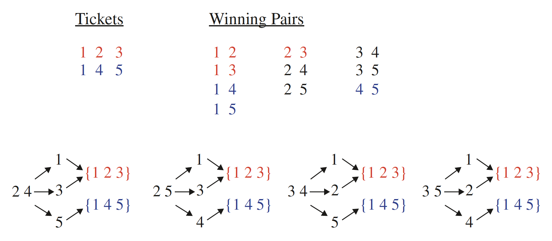
illustrates how we are guaranteed a winning pair from $\{1,2,3,4,5\}$ using only tickets $\{1,2,3\}$ and $\{1,4,5\}$. The bottom figure in the image above shows how all missing pairs imply a covered pair on expansion.

Covered Pairs on Expansion

Although the pairs $\{2,4\}$, $\{2,5\}$, $\{3,4\}$, or $\{3,5\}$ do not explicitly appear in one of the two tickets, these pairs plus any possible third ticket number must create a pair in either $\{1,2,3\}$ or $\{1,4,5\}$. What does this mean and how does the image above help?

In this small example case, since the number of slots for numbers on each ticket is $k=3$, the numbers are chosen distinctly, $n=j=5$, and $S=\{1,2,3,4,5\}$ is our candidate set, this means we can reason as follows:

• If $\{2,4\}$ is a winning pair, then the third number on the winning ticket must come from the set $S\setminus\{2,4\}=\{1,3,5\}$. The winning ticket must then be one of the following:

$$\underbrace{\{{\color{red}{1}},{\color{red}{2}},4\}}_{\color{red}{\{1,2,3\}}},\quad \underbrace{\{{\color{red}{2}},{\color{red}{3}},4\}}_{\color{red}{\{1,2,3\}}},\quad \underbrace{\{2,{\color{blue}{4}},{\color{blue}{5}}\}}_{\color{blue}{\{1,4,5\}}}$$

• If $\{2,5\}$ is a winning pair, then the third number on the winning ticket must come from the set $S\setminus\{2,5\}=\{1,3,4\}$. The winning ticket must then be one of the following:

$$\underbrace{\{{\color{red}{1}},{\color{red}{2}},5\}}_{\color{red}{\{1,2,3\}}},\quad \underbrace{\{{\color{red}{2}},{\color{red}{3}},5\}}_{\color{red}{\{1,2,3\}}},\quad \underbrace{\{2,{\color{blue}{4}},{\color{blue}{5}}\}}_{\color{blue}{\{1,4,5\}}}$$

• If $\{3,4\}$ is a winning pair, then the third number on the winning ticket must come from the set $S\setminus\{3,4\}=\{1,2,5\}$. The winning ticket must then be one of the following:

$$\underbrace{\{{\color{red}{1}},{\color{red}{3}},4\}}_{\color{red}{\{1,2,3\}}},\quad \underbrace{\{{\color{red}{2}},{\color{red}{3}},4\}}_{\color{red}{\{1,2,3\}}},\quad \underbrace{\{3,{\color{blue}{4}},{\color{blue}{5}}\}}_{\color{blue}{\{1,4,5\}}}$$

• If $\{3,5\}$ is a winning pair, then the third number on the winning ticket must come from the set $S\setminus\{3,5\}=\{1,2,4\}$. The winning ticket must then be one of the following:

$$\underbrace{\{{\color{red}{1}},{\color{red}{3}},5\}}_{\color{red}{\{1,2,3\}}},\quad \underbrace{\{{\color{red}{2}},{\color{red}{3}},5\}}_{\color{red}{\{1,2,3\}}},\quad \underbrace{\{3,{\color{blue}{4}},{\color{blue}{5}}\}}_{\color{blue}{\{1,4,5\}}}$$

The purpose of the argument above is to show how all missing pairs imply that a prize-winning pair is still implicitly covered by either $\{1,2,3\}$ or $\{1,4,5\}$. Color coding is used above to make the association clear between the ticket covering the prize-winning pair that results from a missing pair being on a winning ticket.

The general outline of Skiena's search-based solution still held for the real problem. All that needed fixing was identifying which subsets they got credit for covering with a given set of tickets. Skiena credits recovery from this initial error to the basic correctness of the initial formulation, and the use of well-defined abstractions for such tasks as (1) ranking/unranking $k$-subsets, (2) the set data structure, and (3) combinatorial search.

Take-home lessons

Algorithms vs. heuristics

There is a fundamental difference between algorithms, procedures that always produce a correct result, and heuristics, which may usually do a good job but provide no guarantee of correctness. [3]

Importance of proof

Reasonable-looking algorithms can easily be incorrect. Algorithm correctness is a property that must be carefully demonstrated. [3]

Narrow allowable instances

An important and honorable technique in algorithm design is to narrow the set of allowable instances until there is a correct and efficient algorithm. For example, we can restrict a graph problem from general graphs down to trees, or a geometric problem from two dimensions down to one. [3]

The heart of an algorithm is its idea

The heart of any algorithm is an idea. If your idea is not clearly revealed when you express an algorithm, then you are using too low-level a notation to describe it. [3]

For example, the pseudocode

% page 8 of Algorithm Design Manual
\begin{algorithm}
\caption{Exhaustive Scheduling}
\begin{algorithmic}
\PROCEDURE{ExhaustiveScheduling}{$I$}
\STATE $j=0$
\STATE $S_{\max}=\emptyset$
\FOR{each of the $2^n$ subsets $S_i$ of intervals $I$}
  \IF{($S_i$ is mutually non-overlapping) and ($\operatorname{size}(S_i)>j$)}
    \STATE $j=\operatorname{size}(S_i)$
    \STATE $S_{\max}=S_i$
  \ENDIF
\ENDFOR
\RETURN $S_{\max}$
\ENDPROCEDURE
\end{algorithmic}
\end{algorithm}

could be more clearly expressed as

% page 8 of Algorithm Design Manual
\begin{algorithm}
\caption{Exhaustive Scheduling (Revised)}
\begin{algorithmic}
\PROCEDURE{ExhaustiveScheduling}{$I$}
\STATE Test all $2^n$ subsets of intervals from $I$.
\RETURN the largest subset consisting of mutually non-overlapping intervals.
\ENDPROCEDURE
\end{algorithmic}
\end{algorithm}

Disprove heuristics with counterexamples

Searching for counterexamples is the best way to disprove the correctness of a heuristic. [3]

Inductively verify recursive or incremental algorithms

Mathematical induction is usually the right way to verify the correctness of a recursive or incremental insertion algorithm. [3]

Model applications in terms of well-defined structures

Modeling your application in terms of well-defined structures and algorithms is the most important single step towards a solution.